| prev | home | next |
In this instalment of the Physics of Racing, we complete the program begun last time to combine the magic formulae of parts 21 and 22, so that we have a model of tire forces when turning and braking or turning and accelerating at the same time. Parts 21 and 22 introduced the magic formulae. The first one takes longitudinal slip as input and produces longitudinal grip as output. The other one takes lateral slip as input and produces lateral grip. Slip depends primarily on driver inputs, grip is force generated at the ground. Longitudinal means in the straight-ahead direction. Lateral means sideways, as in the forces for turning. Since the magic formulae work only in isolation, we have work to do to model turning and braking at the same time and turning and accelerating at the same time.
Last time, we vectorized slip - the input - to come up with combination slip, captured in the vector slip velocity. That vector measures the velocity of the contact patch with respect to (w.r.t.) the ground in one, handy definition. This time, we first boil down combination slip to new inputs for the old magic formulae. In the old magic formulae, we measure longitudinal slip as a percentage of unity, that is, as a percentage of breakaway sliding; and we measure lateral slip as an angle in degrees. These are not commensurable, meaning that we do not use the same units of measurement for both kinds of slip. That's why there was a big, fat question mark in the vector slot for combination slip in one of the tables in part 24. Once we make them commensurable, then we stitch the magic formulae together to get one vector gripping force as a function of one vector slip. This finally allows us to compute the forces delivered by a tire under combination control inputs.
Once again, we are in uncharted territory, so take it all in the for-fun spirit of this whole series of articles. I don't represent anything I do here as authoritative racing practice. I only claim to be bringing the fresh perspective of a stubbornly naïve physicist to the problems of racing cars as an amateur. The standard practice of the professional racing engineering community may be completely different. This is the Physics of Racing, not the Engineering of Racing. I'm after the fundamental principles behind the game. I use techniques that may be foreign to the engineers that build and race cars professionally. My results may not be precise enough for final application. I may take approximations that simplify away things that are actually critically important. On purpose, I'm figuring things out on my own. Often, this helps me understand published engineering information better. Just as often, it helps me debunk and debug the conventional wisdom. If you find mistakes, gaffs, or laughable dumb stuff, or if you know better ways to do things, I encourage you to fire up debate, publish rebuttals, or write to me directly. I've done my best to track down the latest and greatest information, but I've found lots of errors, ambiguities, and inexplicabilities in the open literature. I also suspect a conspiracy, meaning that I'd bet that the tyre manufacturers and pro racing teams don't publish their best information-I certainly wouldn't if I were they.
Disclaimers out of the way, we now have enough tools on the table to combine
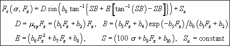
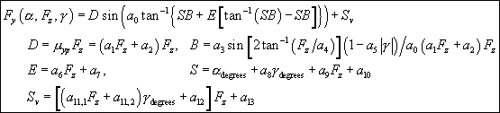
the two magic formulae. Recall the formulae from parts 21 and 22: ![]() and
and
![]() for the longitudinal and lateral forces. Here they are, in isolation:
for the longitudinal and lateral forces. Here they are, in isolation:
There are a lot of ways we could stitch them together. This is not the kind
of situation where there is one right answer. Instead, in the absence of hard
theory or experimental data, we have the freedom to be creative, with the
inevitable risk of being wrong. We pick a method that satisfies some simple,
intuitive, physical requirements. First, we must put the inputs on the same
footing. Ask "what is the value of ![]() for which
for which ![]() has its
maximum, and what is the value of
has its
maximum, and what is the value of ![]() for which
for which ![]() has its
maximum?" Call these two values
has its
maximum?" Call these two values ![]() and
and ![]() . They are
constants for given Fx and
. They are
constants for given Fx and ![]() : characteristics
of a particular tyre and car and surface. So, we can finesse the notation and
just write
: characteristics
of a particular tyre and car and surface. So, we can finesse the notation and
just write ![]() and
and ![]() . The maxima identify points on the rim or edge of the
'traction circle'. The grip decreases when
. The maxima identify points on the rim or edge of the
'traction circle'. The grip decreases when ![]() exceeds
exceeds ![]() and
when
and
when ![]() exceeds
exceeds ![]() . Let's illustrate with
. Let's illustrate with ![]() ,
, ![]() = 0,
and the constants from Genta's alleged Ferrari. Once we substitute all that in
(and we'll let you check our arithmetic from the data in prior articles), we get
= 0,
and the constants from Genta's alleged Ferrari. Once we substitute all that in
(and we'll let you check our arithmetic from the data in prior articles), we get
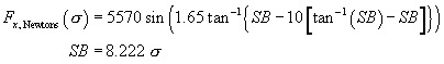
We evaluate these equations for ![]() = 0,
= 0, ![]() = 0, getting
= 0, getting ![]() ,
, ![]() ,
and showing a small lateral force (about 16 lbs) due to conicity and ply steer.
The source of that problem is the constant offset in S, which results
from a9 and a10's being non-zero. We just
set them to zero for now. Let's plot
,
and showing a small lateral force (about 16 lbs) due to conicity and ply steer.
The source of that problem is the constant offset in S, which results
from a9 and a10's being non-zero. We just
set them to zero for now. Let's plot ![]() , slip on the horizontal axis and grip on
the vertical:
, slip on the horizontal axis and grip on
the vertical:
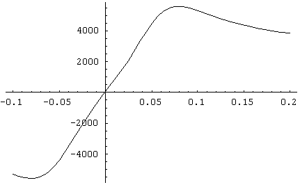
The maximum positive grip occurs, just by eyeball, around ![]() = 0.08. To
the left of the maximum, adding more slip - more throttle - generates more grip.
To the right of the maximum, adding more slip generates less grip.
That's where we've lost traction. We can find the maximum precisely by plotting
the slope of this curve, since the slope is zero right at the maximum:
= 0.08. To
the left of the maximum, adding more slip - more throttle - generates more grip.
To the right of the maximum, adding more slip generates less grip.
That's where we've lost traction. We can find the maximum precisely by plotting
the slope of this curve, since the slope is zero right at the maximum:
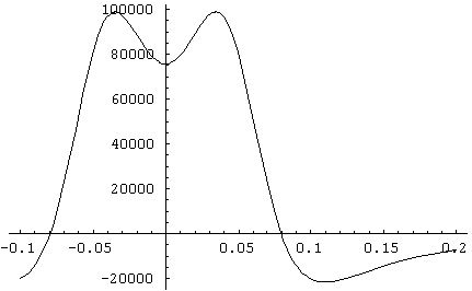
Using secret physicist methods, I've found that this curve crosses the
horizontal axis - that is, goes to zero - at precisely ![]() = 0.0796.
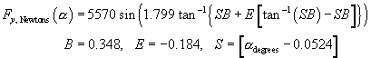
This was so much fun that we'll just do it again for
= 0.0796.
This was so much fun that we'll just do it again for ![]() . First, the
curve proper:
. First, the
curve proper:
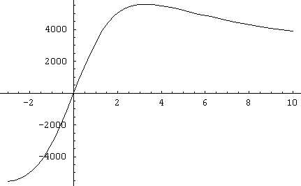
Notice the same kind of stability situation as we saw before. To the left of the maximum, more slip - more steering - means more grip. To the right of the maximum, more slip means less grip. Here's the slope:
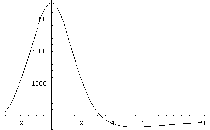
We find that the maximum of the original curve, the zero-crossing of the
slope, occurs at ![]() = 3.273°
= 3.273°
Once we find the maxima, we can create new, non-dimensional quantities by
scaling ![]() and
and ![]() by these values, namely
by these values, namely ![]() . These are
pure numbers, so they're commensurable. They are unity when
. These are
pure numbers, so they're commensurable. They are unity when ![]() and
and ![]() have
the values of maximum traction in isolation of one another. We can then write
new functions
have
the values of maximum traction in isolation of one another. We can then write
new functions ![]() and
and ![]() which have their maxima at s = 1
and a = 1. We seek a vector-valued function
which have their maxima at s = 1
and a = 1. We seek a vector-valued function ![]() of s and
a whose longitudinal x component
of s and
a whose longitudinal x component ![]() expresses the
longitudinal force component and whose lateral y component
expresses the
longitudinal force component and whose lateral y component ![]() expresses the
lateral force component under combination slip. Build this up from
expresses the
lateral force component under combination slip. Build this up from ![]() and
and ![]() so
that it satisfies the following requirements:
so
that it satisfies the following requirements:
The following table fleshes out requirement 3 for the cases of braking (![]() < 0
) or turning left (
< 0
) or turning left (![]() < 0 ). The essential idea is that if the magnitude of
either parameter increases, then the magnitudes of the inputs to the old magic
formulae must increase, but honouring the algebraic signs. If a parameter is
positive, it should get more positive as the magnitude of the other parameter
increases. Similarly, if a parameter is negative, it should get more negative as
the magnitude of the other parameter increases.
< 0 ). The essential idea is that if the magnitude of
either parameter increases, then the magnitudes of the inputs to the old magic
formulae must increase, but honouring the algebraic signs. If a parameter is
positive, it should get more positive as the magnitude of the other parameter
increases. Similarly, if a parameter is negative, it should get more negative as
the magnitude of the other parameter increases.
| sgn( |
sgn( |
input to Fx | input to Fy | ||
|---|---|---|---|---|---|
| + | + | increasing | fixed | increasing | increasing |
| + | + | fixed | increasing | increasing | increasing |
| + | - | increasing | fixed | increasing | decreasing |
| + | - | fixed | decreasing | increasing | decreasing |
| - | + | decreasing | fixed | decreasing | increasing |
| - | + | fixed | increasing | decreasing | increasing |
| - | - | decreasing | fixed | decreasing | decreasing |
| - | - | fixed | decreasing | decreasing | decreasing |
Without further ado, here's our proposal for the combination magic grip formula:
|
|
Using ![]() as the input, with the appropriate algebraic signs, satisfies
requirements 1. Multiplying the outputs by the ratio of s to
as the input, with the appropriate algebraic signs, satisfies
requirements 1. Multiplying the outputs by the ratio of s to ![]() and a
to
and a
to ![]() magically satisfies requirements 2, 3, and 4. There is, in fact, plenty of
freedom in the choice of the outer multiplier: strictly speaking, any power of
the ratios would do for requirements 2 and 4, and some care will be required to
get the signs right for requirement 3. Until we have a good reason to change it,
we'll just go with the ratio straight up, especially since it
automatically gets the signs right. We close this instalment with a plot of the
magnitude
magically satisfies requirements 2, 3, and 4. There is, in fact, plenty of
freedom in the choice of the outer multiplier: strictly speaking, any power of
the ratios would do for requirements 2 and 4, and some care will be required to
get the signs right for requirement 3. Until we have a good reason to change it,
we'll just go with the ratio straight up, especially since it
automatically gets the signs right. We close this instalment with a plot of the
magnitude ![]() showing the traction circle very clearly:
showing the traction circle very clearly:
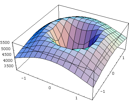
The stability criteria are visually obvious, here. If the current, commensurable slip values, s and a, are inside the central "cup" region, then increasing either component of slip increases grip. If they're outside, then increasing slip leads to decreasing grip and the driver is in the "deep kimchee" region of the plot.
| ERRATA: The Physics of Racing series has been fairly error-free over the years, but I caught three small errors in part 22 whilst going over it for this instalment. The good news is that they did not affect any final results. I defined the WHEEL frame at the wheel hub but later I implied that it is centred at the contact patch (CP). In fact, the frame at the CP is the important one, and we call it TYRE from now on, avoiding the ambiguous "WHEEL". We never actually used the improperly defined WHEEL frame, so, again, final results were not affected. Also, the dimensions for a3 in Part 22 should be N/Degree, not just N, because a3 furnishes the dimensions for B, which always appears in the combination SB, and has dimensions of degrees. Finally, the dimensions for a6 are 1/KN, not KN. |